Signal Theory and Convolution

Convolution is a key to deciphering various aspects of signal theory. This concept is often left to its theoretical analysis and analytical perplexity. This is an attempt to illuminate this beautiful concept with some intuitive examples and explanations.

Central limit theorem

Introduction

Signals are waves that carry information. Anything that accepts signal as an input and gives an output is a system. In a broad sense, systems allows signals to propagate through them. For e.g. a wire carrying electrical current is a system. Systems process and transform the signal as it passes through them. Here, for brevity we will consider systems that have linear behavior and do not change with time. The category of systems is known as Linear Time Invariant (LTI) systems.

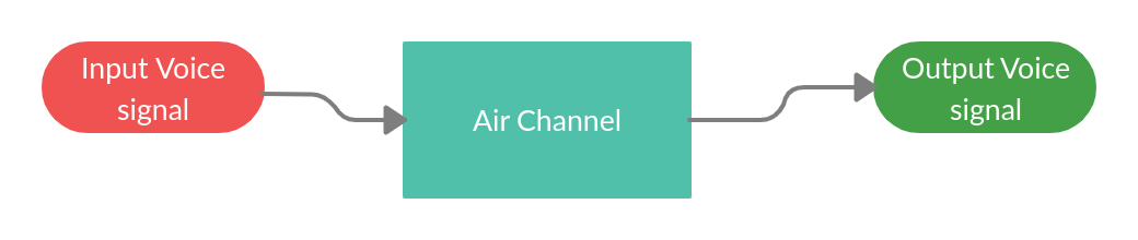
Let’s consider a familiar scenario– when two people talk, the person speaking generates an input voice signal, and the air channel b/w the two participants act as a system.

converation — **Fig 1:** An exemplary conversation

The voice signal flows through the air channel and is received by the listener. The air channel alters the voice signal by adding distortions and noise, i.e. the received voice signal is slighlty different than the original one.

signal System — **Fig 2:** System input output

It is often desired to model and understand the behavior of these systems. The idea is that, if we can somehow determine the equation governing the system, it would allow us to evaluate the behavior of the system for different types of signals. We can evaluate the effect of the channel on say, on WiFi signals, or blue-tooth signals. Further, this analysis can greatly help engineers in design of communication systems.

Impulse response to Convolution

The evaulation of equation governing a system might seem a challenging task. Surprisingly, there exist an interesting and simple approach to this problem. It turns out, when a system provided with impulse function as an input produces its equation as an output. This response(or output) of the system, measured using an impulse signal, is known as the Impulse response of the system.

\[\begin{align*} & h(t) = x(t) \ast h(t)\\ where, \\ & x(t)=\delta(t) \\ \end{align*}\]

The \(\ast\) operator is used to denote convolution operation. And, convolution of an impulse signal \(\delta(t)\) with system \(h(t)\) is known as the impulse response. We can think impulse function as an arrow to capture the characteristics of a system, which is otherwise not known.

We can verify this fact in few lines of python code:

The output looks like this:

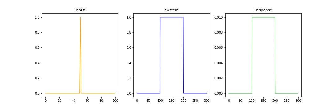
impulse response — **Fig 3:** Convolution of an impulse with a system

Here, the output of the system is given as convolution of input signal \(h(t)\) with system equation. The convolution of signal \(x(t)\) with system \(h(t)\) is defined as:

\[\begin{align*} & \phi(t) = x(t) \ast h(t)\\ & \phi(t) = \int_{-\infty}^\infty x(\tau) h(t-\tau)d\tau \\ \end{align*}\]

Under the hood, the operation simplifies to flipping one of the signals and sweeping it across the entire range, evaluating the area of the overlapping region. The two fundamental operations at play are shifting and adding. These two fundamental operations appear in all forms of convolution operation. This is depicted in the following animation from Wikipedia.

Notice, how one signal changes and tries to capture some of the features of the another. The essence of convolution operation lies in capturing the behavior of the system and applying them to input signals to derive the output is signal. Hence, the output signal adorns the characteristics of the system.

Practical aspects of Convolution

Convolution is an essential operation in audio signal processing where the process is used to generate different sound effects in the multimedia industry. Here are two examples from CKSDE which allows you to listen to the convolution of two different audio samples.

Example 1.1:

In this example, voice of a man is fed as an input to a system that produces a metallic delay effect.

Example 1.2:

In this example, audio of a snare drum is fed as an input to a system that produces a decaying white noise.

Apart from this, convolutions also work with images and have immense applications in image recognition, filtering, etc. These are some interesting topics, which I would cover separately in my future posts.

Example 2:

Image processing is another domain that witnesses huge application of convolution. Instead of having a signal/system, we have an input image(signal) and an image kernel (system). Images and the image kernel are nothing but matrices with each pixel denoted by a number (or a set of numbers in case of colored images). The image kernel (also known as filters) is a matrix (usually smaller than your image) used to apply effects on an image such as blurring, sharpening, outlining etc.

Here as well, the convolution operation involves shifting and adding. The kernel slides over the image, element-wise multiplications are performed with the pixels of the image, and lastly the sum of these multiplications becomes a pixel of the output/filtered image.

Given below is an example of convolution operation between two matrices:

\[\begin{align*} & \left( \begin{array}{ccc} 3 & 3 & 2 & 1 & 0 \\ 0 & 0 & 1 & 3 & 1 \\ 3 & 1 & 2 & 2 & 3 \\ 2 & 0 & 0 & 2 & 2 \\ 2 & 0 & 0 & 0 & 1 \end{array} \right) \ast \left( \begin{array}{c} 0 & 1 & 2 \\ 2 & 2 & 0 \\ 0 & 1 & 2 \end{array} \right) = \left( \begin{array}{c} 12 & 12 & 17 \\ 10 & 17 & 19 \\ 9 & 6 & 14 \end{array} \right) \end{align*}\]

This same techniques can be applied to images as follows in python:

Here, we convolved the image with an outline filter: \(\begin{pmatrix}-1 & -1 & -1 \\ -1 & 8 & -1 \\-1 & -1 & -1 \end{pmatrix}\).

The output shall generate two following images:

Fig 6: Left: Input image. Right: Filtered image

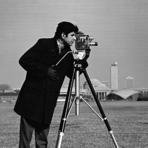
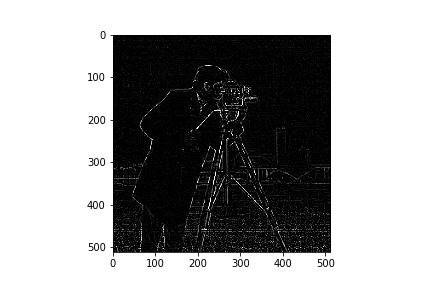
The behavior of the filter can be understood by observing that sum of all the elements of the matrix is zero. If the image is smooth i.e. no changes in color, the convolution output of filter will be zero. But, if there is a sharp change in color gradient (in case of an edge), the output is non-zero. In this way the filter is able to achieve the outline of an image.

The convolution operation beautifully scales from the field of signal processing to neural networks. Convolution is at the heart of some of the most complex yet profound applications such as self driving cars, face recognition used in face unlock, cancer detection, etc.

These applications are possible using the idea of convolution that explores building deep learning models to classify images and identify objects. This class of deep learning models known as Convolutional Neural Networks (or CNN or ConvNets).

CNN are further being used in text to speech synthesis to mimic human voice. This pictionary game uses CNN. Make sure you do not miss CNN being used in autonomous drone.

Ankit Kumar