
Fourier Series with Python
The following post is an effort to provide an intuitive understanding of one of the most popular expansions in mathematics known as the Fourier series.

“There cannot be a language more universal and more simple, more free from errors and obscurities … Mathematical analysis is as extensive as nature itself, and it defines all perceptible relations.” ―Joseph Fourier, The Analytical Theory of Heat
History
Baron Jean-Baptiste Joseph Fourier (1768−1830) was a French mathematician, known for his contributions in the field of heat transfer and the study of vibrations. He also helped develop many mathematical tools with profound applications in today’s world.
He famously pointed out that every periodic function can be made using a combination of sines and cosines. This idea of representing signals as a superposition of basic waves is known as the Fourier series. The idea led to the development of a new branch of mathematics known as harmonic analysis.
Definition
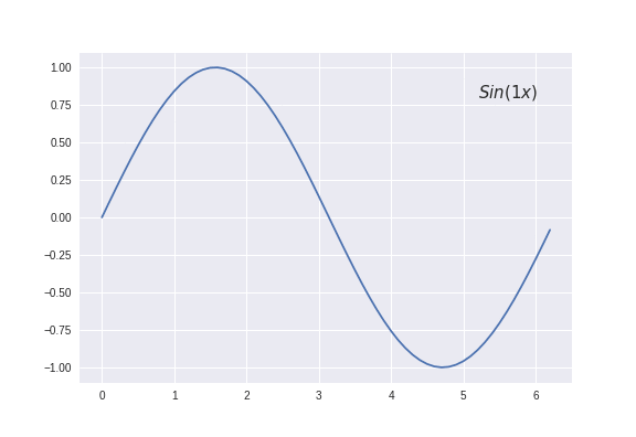
Before jumping right into the mathematical expression of Fourier series, it’s worth spending some time pondering upon a series being a combination of sines and cosines. We know that \(sin(nx)\) and \(cos(nx)\) are periodic functions of period \(\frac{2\pi}{n}\). This implies that the period of these functions can vary for different values of ‘n’.
These sine and cosine functions with different values of ‘n’ are often termed harmonics of the function. For example, \(sin(x)\), \(sin(2x)\), \(sin(3x)\)…, are different harmonics of a sine wave.
Analytically, the Fourier series of a periodic function \(\phi(x)\) with period T is defined as the sum of different harmonics of sines and cosines:
\[\begin{align*} & \phi(x) = a_0+ \sum_{i=1}^\infty a_ncos(nx) + \sum_{i=1}^\infty b_nsin(nx) \\ where,\\ & a_0= \frac{1}{T}\int_0^T\phi(x)dx; \\ & a_n = \frac{2}{T}\int_0^T\phi(x)cos(nx) dx; \\ & b_n = \frac{2}{T}\int_0^T\phi(x)sin(nx) dx; \\ \end{align*}\]Analysis
So far, we have looked at the definition of the Fourier series; now it’s time to get visual intuition using Python. It’s normal to have a counter-intuitive feeling about Fourier series. Especially, it is difficult to visualize a square wave (non-continuous function) being synthesized using sines and cosines (continuous functions). In the following section, we’ll try to visualize the same.
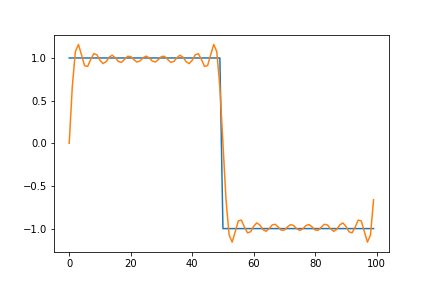
Fourier series for a square wave \(\beta(x)\) with period T is given as:
\[\begin{align*} \beta(x) = \frac{4}{\pi} \sum_{n=1,3,5...}^\infty \frac{1}{n}sin(\frac{n\pi x}{T}) \end{align*}\]Here, we implement a function to generate the Fourier series of a square wave using the expression above. The function takes the number of terms to generate as an input.
The output should look like this:
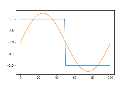
Below is an animated version showing a square function being synthesized by a combination of sine waves. The graph on the left plots each term of the series individually, while the one on the right gives a remarkable view of how the components add up.

Here, we notice that the approximation overshoots the desired value at the edges of the square wave. This peculiar behavior of the Fourier series is known as the Gibbs phenomenon. Informally, the Gibbs phenomenon reflects the difficulty inherent in approximating a discontinuous function by a finite series of continuous sine and cosine waves.
Applications
So, why study Fourier series? Apart from its analytical rigor and visual beauty, does it add something more to this world? Much of our knowledge of the world is contained in functions, so it becomes inevitable that we understand them. The voltage produced by a microphone, as a function of time, represents music that can then be encoded digitally and stored on a compact disc. The position of a planet, as a function of time, represents an orbit.
Functions are everywhere. They are also extremely complex objects. As with the square wave as a function of sine and cosine, any sufficiently complex object is too difficult to comprehend in one glance, for our minds are limited. We therefore study functions from many vantage points and use multiple representations and transforms, such as Fourier series, to generate alternative representations of functions.
Fourier series, in short, tell us what harmonics or frequencies are present in a signal, which can be used to design various filters, compress data, and so on. Although the original motivation of the Fourier series was to solve heat equations, today it has many applications in electrical engineering, vibration analysis, acoustics, optics, signal processing, image processing, etc.
Further exploration
Interested in exploring Fourier series? Check out this video by 3B1B. A detailed analytical introduction to the topic can be studied at Khan Academy.
If you are interested in my work and thoughts, check out my Twitter or connect with me on LinkedIn.