Sampling the World

In this fast-paced world of digital signals, the following article provides a brief moment to pause and ponder upon the concepts that serve as cornerstones of digitization.

sampling_gif

History: An Analog Road to the Digital World

Our world is inherently analog. All naturally occurring information is in the form of analog signals or waves. The sound waves generated by our voice box as we speak or the optical signals perceived by our eyes carry information in a continuous fabric of time and space, hence are analog. The nature of analog signals inspired various early techniques for recording and transmission of information.

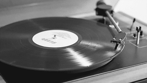
sine_wave — **Fig 1:** An exemplary analog sine wave

The magnetic tape recorders or vinyl records (shown below) were some of the primitive analog methods for data recording. Similarly, early AM and FM systems were purely analog. The early telephone system, which was designed primarily to transmit the human voice, translated sound waves into analog signals for transmission, which were then reconverted into sound waves at the receiving handset.

The process of recording an analog signal may cause significant loss of information. The loss continues as we create more copies from the original recordings. For example, the quality of an originally recorded vinyl would be much higher than its copy. This is similar to creating a xerox copy. The first copy is slightly less bright than the original, and the subsequent copy printed using the first copy has further reduction in quality. Hence, each step incurs loss of information.

Another problem with analog signals is that they are prone to electronic noise and distortion. These distortions are introduced by communication channels and signal processing operations, which can progressively degrade the signal. In contrast, converting an analog signal to digital form introduces low-level quantization noise (discussed later) into the signal. However, once in digital form, the signal can be processed or transmitted without introducing significant additional noise or distortion. In addition, digital systems allow degradation detection and correction, which is not available in analog systems.

These benefits of digital signals over analog drove innovation towards a much more promising world of digital information.

The Digital Shift

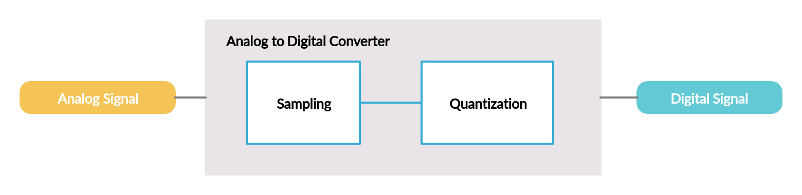
The first step of establishing a digital regime is to invent a device that converts a given analog signal to a digital signal. At the heart of this discretization of signals are devices known as Analog-to-Digital (A/D) converters. These devices serve as a bridge between the two worlds.

An A/D converter converts a continuous-time, continuous-amplitude analog signal (for example, a voice signal entering a microphone or light entering a camera) to a discrete-time, discrete-amplitude digital signal. This conversion involves sampling and quantization of the signal.

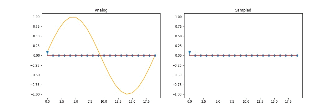
a/d — **Fig 3:** Analog to Digital Converter

Sampling

Sampling is a process of handpicking values out of a continuous range of values. This is done at regular intervals by multiplying the entire signal with a train of impulses.

\[y[n]_{sampled} = x(t)_{analog} \times \sum_{\tau=-\infty}^{\infty} \delta(t-\tau)\tag{1} \label{one}\]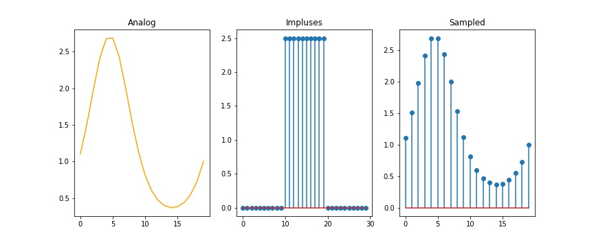

It is quite interesting to look at the sampling operation in the frequency domain. Assume that signal \(x(t)\) has a maximum frequency component as \(w_b\) (\(w=2 \pi f\) where f is the frequency of the signal). When we take the Fourier transform of equation \eqref{one}, we have:

\[\begin{align*} & Y(w)_{sampled} = 1/(2\pi) \times [X(w)_{analog} \ast \sum_{\phi=-\infty}^{\infty} 2\pi \times \delta(w-\phi w_0)]\\ & Y(w)_{sampled} = ...+ X(w+w_0)+ X(w) + X(w-w_0)+ X(w-2w_0)+...\tag{2}\label{two}\\ \end{align*}\]

As shown above in equation \eqref{two}, the frequency component of the signal gets shifted by the impulse train. The various possibilities of shifting in the frequency domain are shown below.

nyquist — **Fig 5:** Sampling at different frequencies

The important thing to observe is that the shifting should be at least twice the maximum frequency component of the signal, i.e., \(w_0 \geq 2w_b\) or \(f_0 \geq 2f_b\). This is known as the Nyquist Criterion. If the relation is not satisfied, the shifted components can interfere with each other. This phenomenon is known as Aliasing. Hence, to avoid aliasing, the sampling of the signal should be at a frequency higher than twice its maximum frequency.

Nyquist theorem or Sampling theorem states that, given a signal with a maximum frequency component of \(f\) Hz, a sampling rate of at least \(2f\) Hz is required to avoid aliasing. This minimum acceptable sampling rate is called the Nyquist rate.

Quantization

After sampling, each sample value is replaced by a binary number. If the sampling frequency is high, the number of samples is higher. And as the number of unique sample values is high, the number of bits required for the representation of the entire signal also increases. Further, a greater number of bits would require more memory space to store the samples. This memory overhead is greatly reduced by the process of quantization.

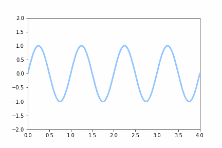
Quantization is the process of mapping continuous infinite values to a smaller set of discrete finite values. In this process, the entire range of the signal is divided into a finite number of levels.

In the example shown below, the sine wave ranges between -4V to 4V. This range is divided into 8 equally spaced levels. Quantization maps every sample to its closest level. For example, \(1.8 \rightarrow 2\), \(0.2 \rightarrow 0\), etc.

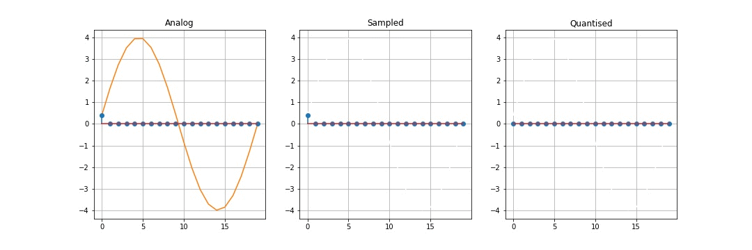
In theory, N unique samples can be represented using n bits if \(2^{n} \geq N\). In this example, there are 20 samples. If we consider the representation of all these samples, it will require 5 bits per sample as \(2^{4}< N<2^{5}\). With 8-level quantization, there are only 8 unique samples which can be represented using 3 bits per sample. This saves 40% memory usage.

But there is no free lunch. The process of quantization approximates original samples to the nearest quantized level, introducing distortions in the original signal. This is known as Quantization Noise or Quantization Error. The reduced memory requirements come at the cost of small distortions in the signal. There are different types of quantizer designs in the industry that aim to reduce the quantization noise to the maximum extent possible. However, the important thing to note is that quantization noise is something that can be reduced but can never be completely eradicated.

Example: Audio Recording

Suppose you wish to record a voice note. The figure below shows a typical setup used for this purpose.

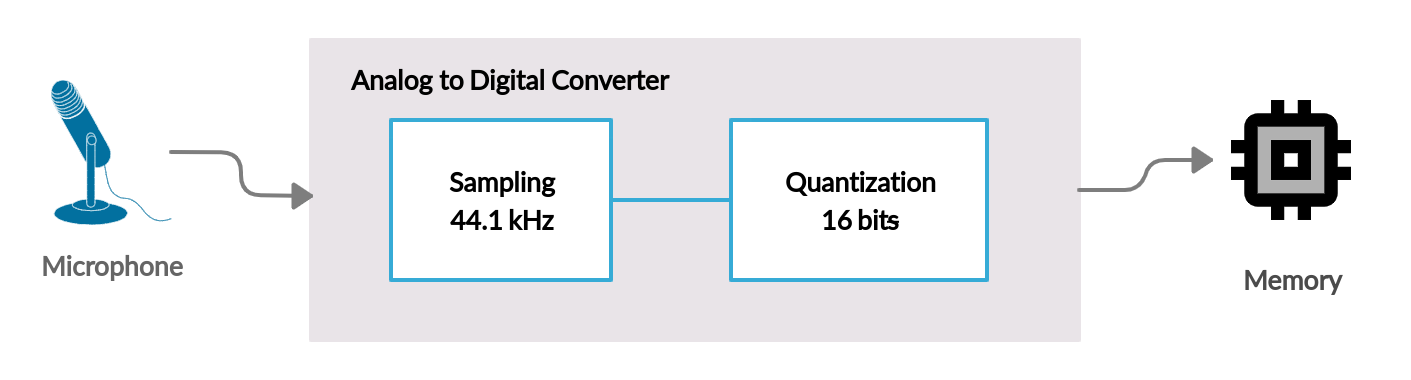
The setup includes a microphone which converts the pressure waves of your voice into analog electrical signals. The microphone is connected to an A/D converter. The output of the A/D converter is a digital stream of bits which is wired into memory for recording.

As human voice typically ranges from 20 Hz to 20 kHz, the sampling rate \((f_s)\) of the A/D converter needs to be more than twice the highest frequency, i.e., \(f_s \geq 40\) kHz. Standard CD-quality audio uses a sample rate of 44.1 kHz. Now we need to decide the number of levels in the quantizer. In the audio industry, this is known as bit depth. Some commonly used audio standards such as MP3 use 8 bits or 16 bits of bit depth.

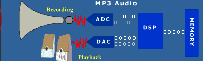
The recorded bits can be retrieved from memory and fed to a digital-to-analog converter software in your phone, which converts it back to an analog signal and outputs it via the speaker. Here’s a picture showing the entire process.

Ankit Kumar